In this article, I am going to discuss Master Theorem. Please read our previous article where we discussed Properties of Asymptotic Notations. Here, you will learn what master theorem is and how it is used for solving recurrence relations.
Master Theorem
The master method is a formula for solving recurrence relations of the form:
T(n) = aT(n/b) + f(n),
where,
n = size of input
a = number of subproblems in the recursion
n/b = size of each subproblem. All subproblems are assumed to have the same size. f(n) = cost of the work done outside the recursive call, which includes the cost of dividing the problem and cost of merging the solutions
Here, a ≥ 1 and b > 1 are constants, and f(n) is an asymptotically positive function. An asymptotically positive function means that for a sufficiently large value of n, we have f(n) > 0.
The master theorem is used in calculating the time complexity of recurrence relations (divide and conquer algorithms) in a simple and quick way.
If a ≥ 1 and b > 1 are constants and f(n) is an asymptotically positive function, then the time complexity of a recursive relation is given by
T(n) = aT(n/b) + f(n)
where, T(n) has the following asymptotic bounds:
1. If f(n) = O(nlogb a-ϵ), then T(n) = Θ(nlogb a).
2. If f(n) = Θ(nlogb a), then T(n) = Θ(nlogb a *log n).
3. If f(n) = Ω(nlogb a+ϵ), then T(n) = Θ(f(n)).
ϵ > 0 is a constant.
Each of the above conditions can be interpreted as:
If the cost of solving the sub-problems at each level increases by a certain factor, the value of f(n) will become polynomially smaller than nlogb a. Thus, the time complexity is oppressed by the cost of the last level ie. nlogb a
If the cost of solving the sub-problem at each level is nearly equal, then the value of f(n) will be nlogb a. Thus, the time complexity will be f(n) times the total number of levels ie. nlogb a* log n
If the cost of solving the subproblems at each level decreases by a certain factor, the value of f(n) will become polynomially larger than nlogb a. Thus, the time complexity is oppressed by the cost of f(n).
Solved Example of Master Theorem
T(n) = 3T(n/2) + n2
Here,
a = 3
n/b = n/2
f(n) = n2
logb a = log2 3 ≈ 1.58 < 2
ie. f(n) < nlogb a+ϵ , where, ϵ is a constant.
Case 3 implies here.
Thus, T(n) = f(n) = Θ(n2)
Master Theorem Limitations
The master theorem cannot be used if:
1. T(n) is not monotone. eg. T(n) = sin n
2. f(n) is not a polynomial. eg. f(n) = 2n
3. a is not a constant. eg. a = 2n
4. a < 1
Master Theorem for Divide and Conquer Recurrences
All divide and conquer algorithms (also discussed in detail in the Divide and Conquer chapter) divide the problem into sub-problems, each of which is part of the original problem, and then perform some additional work to compute the final answer. As an example, a merge sort algorithm [for details, refer to Sorting chapter] operates on two sub-problems, each of which is half the size of the original, and then performs O(n) additional work for merging. This gives the running time equation:
T(n) = 2T(n/2) + O(n)
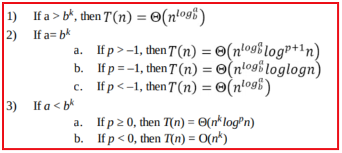
The following theorem can be used to determine the running time of the divide and conquer algorithms. For a given program (algorithm), first, we try to find the recurrence relation for the problem. If the recurrence is of the below form then we can directly give the answer without fully solving it. If the recurrence is of the form ,T(n) = aT (n/b) + Θ(nklogpn) where a ≥ 1,b >1,k ≥ 0 and p is a real number, then:
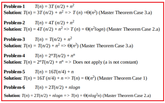
Divide and Conquer Master Theorem: Problems & SolutionsMaster Theorem For each of the following recurrences, give an expression for the runtime T(n) if the recurrence can be solved with the Master Theorem. Otherwise, indicate that the Master Theorem does not apply.
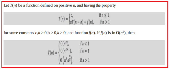
Master Theorem for Subtract and Conquer Recurrences
A variant of Subtraction and Conquer Master Theorem
The solution to the equation T(n) = T(α n) + T((1 – α)n) + βn, where 0 < α < 1 and β > 0 are constants, is O(nlogn).
Method of Guessing and Confirming
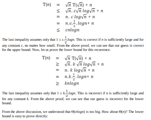
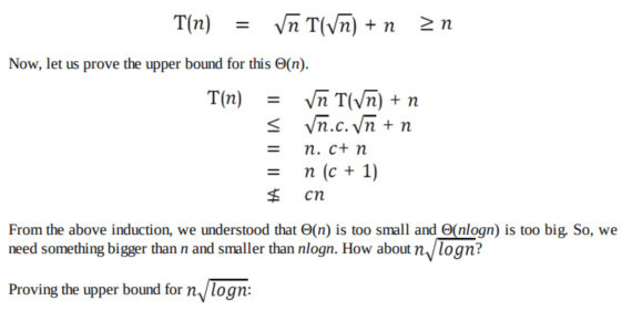
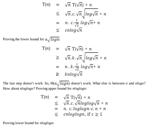
Now, let us discuss a method that can be used to solve any recurrence. The basic idea behind this method is: guess the answer; and then prove it correct by induction.
In other words, it addresses the question: What if the given recurrence doesn’t seem to match with any of these (master theorem) methods? If we guess a solution and then try to verify our guess inductively, usually either the proof will succeed (in which case we are done), or the proof will fail (in which case the failure will help us refine our guess).
Amortized Analysis
Amortized analysis refers to determining the time-averaged running time for a sequence of operations. It is different from average-case analysis because the amortized analysis does not make any assumption about the distribution of the data values, whereas average case analysis assumes the data are not “bad” (e.g., some sorting algorithms do well on average overall input orderings but very badly on certain input orderings). That is, amortized analysis is a worst-case analysis, but for a sequence of operations rather than for individual operations.
The motivation for amortized analysis is to better understand the running time of certain
techniques, where standard worst-case analysis provides an overly pessimistic bound. Amortized analysis generally applies to a method that consists of a sequence of operations, where the vast majority of the operations are cheap, but some of the operations are expensive. If we can show that the expensive operations are particularly rare we can change them to the cheap operations, and only bound the cheap operations.
The general approach is to assign an artificial cost to each operation in the sequence, such that the total of the artificial costs for the sequence of operations bounds the total of the real costs for the sequence. This artificial cost is called the amortized cost of operation. To analyze the running time, the amortized cost thus is a correct way of understanding the overall running time – but note that particular operations can still take longer so it is not a way of bounding the running time of any individual operation in the sequence.
When one event in a sequence affects the cost of later events:
Let us consider an array of elements from which we want to find the k the smallest element. We can solve this problem by using sorting. After sorting the given array, we just need to return the kth element from it. The cost of performing the sort (assuming comparison-based sorting algorithm) is O(nlogn). If we perform n such selections then the average cost of each selection is O(nlogn/n) = O(logn). This clearly indicates that sorting once is reducing the complexity of subsequent operations.
In the next article, I am going to discuss Recursion And BackTracking in detail Here, in this article, I try to explain Master Theorem. I hope you enjoy this Master Theorem article. I would like to have your feedback. Please post your feedback, question, or comments about this article.
Summary:
I hope this post will be helpful to understand the concept of Master Theorem
Please share this post with your friends and colleagues.
For any queries please post a comment below.
Happy Coding 😉
Master Theorem
The master method is a formula for solving recurrence relations of the form:
T(n) = aT(n/b) + f(n),
where,
n = size of input
a = number of subproblems in the recursion
n/b = size of each subproblem. All subproblems are assumed to have the same size. f(n) = cost of the work done outside the recursive call, which includes the cost of dividing the problem and cost of merging the solutions
Here, a ≥ 1 and b > 1 are constants, and f(n) is an asymptotically positive function. An asymptotically positive function means that for a sufficiently large value of n, we have f(n) > 0.
The master theorem is used in calculating the time complexity of recurrence relations (divide and conquer algorithms) in a simple and quick way.
If a ≥ 1 and b > 1 are constants and f(n) is an asymptotically positive function, then the time complexity of a recursive relation is given by
T(n) = aT(n/b) + f(n)
where, T(n) has the following asymptotic bounds:
1. If f(n) = O(nlogb a-ϵ), then T(n) = Θ(nlogb a).
2. If f(n) = Θ(nlogb a), then T(n) = Θ(nlogb a *log n).
3. If f(n) = Ω(nlogb a+ϵ), then T(n) = Θ(f(n)).
ϵ > 0 is a constant.
Each of the above conditions can be interpreted as:
If the cost of solving the sub-problems at each level increases by a certain factor, the value of f(n) will become polynomially smaller than nlogb a. Thus, the time complexity is oppressed by the cost of the last level ie. nlogb a
If the cost of solving the sub-problem at each level is nearly equal, then the value of f(n) will be nlogb a. Thus, the time complexity will be f(n) times the total number of levels ie. nlogb a* log n
If the cost of solving the subproblems at each level decreases by a certain factor, the value of f(n) will become polynomially larger than nlogb a. Thus, the time complexity is oppressed by the cost of f(n).
Solved Example of Master Theorem
T(n) = 3T(n/2) + n2
Here,
a = 3
n/b = n/2
f(n) = n2
logb a = log2 3 ≈ 1.58 < 2
ie. f(n) < nlogb a+ϵ , where, ϵ is a constant.
Case 3 implies here.
Thus, T(n) = f(n) = Θ(n2)
Master Theorem Limitations
The master theorem cannot be used if:
1. T(n) is not monotone. eg. T(n) = sin n
2. f(n) is not a polynomial. eg. f(n) = 2n
3. a is not a constant. eg. a = 2n
4. a < 1
Master Theorem for Divide and Conquer Recurrences
All divide and conquer algorithms (also discussed in detail in the Divide and Conquer chapter) divide the problem into sub-problems, each of which is part of the original problem, and then perform some additional work to compute the final answer. As an example, a merge sort algorithm [for details, refer to Sorting chapter] operates on two sub-problems, each of which is half the size of the original, and then performs O(n) additional work for merging. This gives the running time equation:
T(n) = 2T(n/2) + O(n)
The following theorem can be used to determine the running time of the divide and conquer algorithms. For a given program (algorithm), first, we try to find the recurrence relation for the problem. If the recurrence is of the below form then we can directly give the answer without fully solving it. If the recurrence is of the form ,T(n) = aT (n/b) + Θ(nklogpn) where a ≥ 1,b >1,k ≥ 0 and p is a real number, then:
Divide and Conquer Master Theorem: Problems & SolutionsMaster Theorem For each of the following recurrences, give an expression for the runtime T(n) if the recurrence can be solved with the Master Theorem. Otherwise, indicate that the Master Theorem does not apply.
Master Theorem for Subtract and Conquer Recurrences
A variant of Subtraction and Conquer Master Theorem
The solution to the equation T(n) = T(α n) + T((1 – α)n) + βn, where 0 < α < 1 and β > 0 are constants, is O(nlogn).
Method of Guessing and Confirming
Now, let us discuss a method that can be used to solve any recurrence. The basic idea behind this method is: guess the answer; and then prove it correct by induction.
In other words, it addresses the question: What if the given recurrence doesn’t seem to match with any of these (master theorem) methods? If we guess a solution and then try to verify our guess inductively, usually either the proof will succeed (in which case we are done), or the proof will fail (in which case the failure will help us refine our guess).
Amortized Analysis
Amortized analysis refers to determining the time-averaged running time for a sequence of operations. It is different from average-case analysis because the amortized analysis does not make any assumption about the distribution of the data values, whereas average case analysis assumes the data are not “bad” (e.g., some sorting algorithms do well on average overall input orderings but very badly on certain input orderings). That is, amortized analysis is a worst-case analysis, but for a sequence of operations rather than for individual operations.
The motivation for amortized analysis is to better understand the running time of certain
techniques, where standard worst-case analysis provides an overly pessimistic bound. Amortized analysis generally applies to a method that consists of a sequence of operations, where the vast majority of the operations are cheap, but some of the operations are expensive. If we can show that the expensive operations are particularly rare we can change them to the cheap operations, and only bound the cheap operations.
The general approach is to assign an artificial cost to each operation in the sequence, such that the total of the artificial costs for the sequence of operations bounds the total of the real costs for the sequence. This artificial cost is called the amortized cost of operation. To analyze the running time, the amortized cost thus is a correct way of understanding the overall running time – but note that particular operations can still take longer so it is not a way of bounding the running time of any individual operation in the sequence.
When one event in a sequence affects the cost of later events:
-
One particular task may be expensive.
But it may leave data structure in a state that the next few operations become easier.
Let us consider an array of elements from which we want to find the k the smallest element. We can solve this problem by using sorting. After sorting the given array, we just need to return the kth element from it. The cost of performing the sort (assuming comparison-based sorting algorithm) is O(nlogn). If we perform n such selections then the average cost of each selection is O(nlogn/n) = O(logn). This clearly indicates that sorting once is reducing the complexity of subsequent operations.
In the next article, I am going to discuss Recursion And BackTracking in detail Here, in this article, I try to explain Master Theorem. I hope you enjoy this Master Theorem article. I would like to have your feedback. Please post your feedback, question, or comments about this article.
Summary:
I hope this post will be helpful to understand the concept of Master Theorem
Please share this post with your friends and colleagues.
For any queries please post a comment below.
Happy Coding 😉





0 comments:
Post a Comment
If you like this website, please share with your friends on Facebook, Twitter, LinkedIn.