• Home
  • About
  • Contact
  • ado.net
  • angular
  • c#.net
  • design patterns
  • linq
  • mvc
  • .net core
    • .Net Core MVC
    • Blazor Tutorials
  • sql
  • web api
  • dotnet
    • SOLID Principles
    • Entity Framework
    • C#.NET Programs and Algorithms
  • Others
    • C# Interview Questions
    • SQL Server Questions
    • ASP.NET Questions
    • MVC Questions
    • Web API Questions
    • .Net Core Questions
    • Data Structures and Algorithms
Showing posts with label Data Structure. Show all posts

Wednesday, August 5, 2020

Recursion And Back Tracking

 Admin     August 05, 2020     Algorithm, Data Structure     No comments   

In this article, I am going to discuss Recursion And BackTracking in detail. Please read our previous article where we discussed Master Theorem. In this article, we will look at one of the important topics, “recursion”, which will be used in almost every chapter, and also its relative “backtracking”.

What is Recursion?
Any function which calls itself is called recursive. A recursive method solves a problem by calling a copy of itself to work on a smaller problem. This is called the recursion step. The recursion step can result in many more such recursive calls.

It is important to ensure that the recursion terminates. Each time the function calls itself with a slightly simpler version of the original problem. The sequence of smaller problems must eventually converge on the base case.

Why Recursion?
Recursion is a useful technique borrowed from mathematics. Recursive code is generally shorter and easier to write than iterative code. Generally, loops are turned into recursive functions when they are compiled or interpreted.

Recursion is most useful for tasks that can be defined in terms of similar sub-tasks. For example, sort, search, and traversal problems often have simple recursive solutions.

Format of a Recursive Function
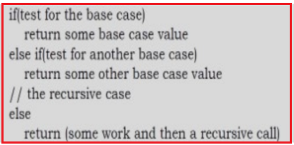
A recursive function performs a task in part by calling itself to perform the subtasks. At some point, the function encounters a subtask that it can perform without calling itself. This case, where the function does not recur, is called the base case. The former, where the function calls itself to perform a subtask, is referred to as the recursive case. We can write all recursive functions using the format:
Recursion And Back Tracking

As an example consider the factorial function: n! is the product of all integers between n and 1.The definition of recursive factorial looks like:
Recursion And Back Tracking

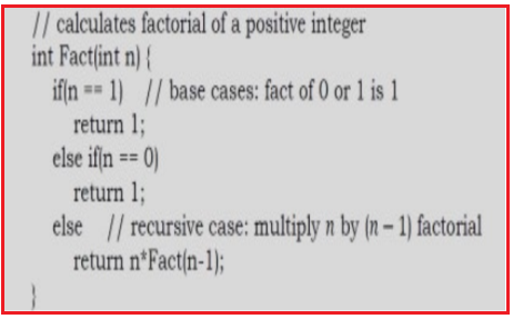
This definition can easily be converted to recursive implementation. Here the problem is determining the value of n!, and the subproblem is determining the value of (n – l)!. In the recursive case, when n is greater than 1, the function calls itself to determine the value of (n – l)! and multiplies that with n.

In the base case, when n is 0 or 1, the function simply returns 1. This looks like the following:
Recursion And Back Tracking

Recursion and Memory (Visualization)
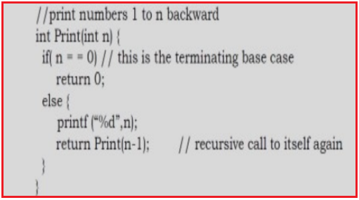
Each recursive call makes a new copy of that method (actually only the variables) in memory. Once a method ends (that is, returns some data), the copy of that returning method is removed from memory. The recursive solutions look simple but visualization and tracing take time. For better understanding, let us consider the following example.
Recursion And Back Tracking

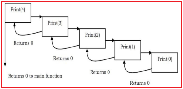
For this example, if we call the print function with n=4, visually our memory assignments may look like:
Recursion And Back Tracking

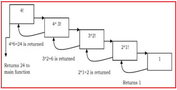
Now, let us consider our factorial function. The visualization of factorial function with n=4 will look like:
Recursion And Back Tracking

Recursion versus Iteration
While discussing recursion, the basic question that comes to mind is: which way is better? –iteration or recursion? The answer to this question depends on what we are trying to do. A recursive approach mirrors the problem that we are trying to solve. A recursive approach makes it simpler to solve a problem that may not have the most obvious of answers. But, recursion adds overhead for each recursive call (needs space on the stack frame).

Recursion
  1. Terminates when a base case is reached.
  2. Each recursive call requires extra space on the stack frame (memory).
  3. If we get infinite recursion, the program may run out of memory and result in stack overflow.
  4. Solutions to some problems are easier to formulate recursively.
Iteration
  1. Terminates when a condition is proven to be false.
  2. Each iteration does not require extra space.
  3. An infinite loop could loop forever since there is no extra memory being created.
  4. Iterative solutions to a problem may not always be as obvious as a recursive solution.
Notes on Recursion
  1. Recursive algorithms have two types of cases, recursive cases, and base cases.
  2. Every recursive function case must terminate at a base case.
  3. Generally, iterative solutions are more efficient than recursive solutions [due to the overhead of function calls].
  4. A recursive algorithm can be implemented without recursive function calls using a stack, but it’s usually more trouble than its worth. That means any problem that can be solved recursively can also be solved iteratively.
  5. For some problems, there are no obvious iterative algorithms.
  6. Some problems are best suited for recursive solutions while others are not.
Example Algorithms of Recursion
  1. Fibonacci Series, Factorial Finding
  2. Merge Sort, Quick Sort
  3. Binary Search
  4. Tree Traversals and many Tree Problems: InOrder, PreOrder PostOrder
  5. Graph Traversals: DFS [Depth First Search] and BFS [Breadth First Search]
  6. Dynamic Programming Examples
  7. Divide and Conquer Algorithms
  8. Towers of Hanoi
  9. Backtracking Algorithms [we will discuss in the next section]
Recursion: Problems & Solutions
In this chapter, we cover a few problems with recursion and we will discuss the rest in other chapters. By the time you complete reading the entire book, you will encounter many recursion problems.

Problem-1 Discuss Towers of Hanoi puzzle.
Solution: The Towers of Hanoi is a mathematical puzzle. It consists of three rods (or pegs or towers), and a number of disks of different sizes which can slide onto any rod. The puzzle starts with the disks on one rod in ascending order of size, the smallest at the top, thus making a conical shape. The objective of the puzzle is to move the entire stack to another rod, satisfying the following rules:
  1. Only one disk may be moved at a time.
  2. Each move consists of taking the upper disk from one of the rods and sliding it onto
another rod, on top of the other disks that may already be present on that rod. No disk may be placed on top of a smaller disk.

Algorithm:
  1. Move the top n – 1 disk from Source to Auxiliary tower,
  2. Move the nth disk from Source to Destination tower,
  3. Move the n – 1 disks from Auxiliary tower to Destination tower.
  4. Transferring the top n – 1 disks from Source to Auxiliary tower can again be thought of as a fresh problem and can be solved in the same manner. Once we solve Towers of Hanoi with three disks, we can solve it with any number of disks with the above algorithm.

Recursion And Back Tracking

Problem-2: Given an array, check whether the array is in sorted order with recursion.
Solution:
Recursion And Back Tracking

Time Complexity: O(n). Space Complexity: O(n) for recursive stack space.

What is Backtracking?
Backtracking is an improvement of the brute force approach. It systematically searches for a solution to a problem among all available options. In backtracking, we start with one possible option out of many available options and try to solve the problem if we are able to solve the problem with the selected move then we will print the solution else we will backtrack and select some other option and try to solve it. If none of the options work out we will claim that there is no solution for the problem.

Backtracking is a form of recursion. The usual scenario is that you are faced with a number of options, and you must choose one of these. After you make your choice you will get a new set of options; just what set of options you get depends on what choice you made. This procedure is repeated over and over until you reach a final state. If you made a good sequence of choices, your final state is a goal state; if you didn’t, it isn’t.

Backtracking can be thought of as a selective tree/graph traversal method. The tree is a way of representing some initial starting position (the root node) and a final goal state (one of the leaves). Backtracking allows us to deal with situations in which a raw brute-force approach would explode into an impossible number of options to consider. Backtracking is a sort of refined brute force. At each node, we eliminate choices that are obviously not possible and proceed to recursively check only those that have potential.

What’s interesting about backtracking is that we back up only as far as needed to reach a previous decision point with an as-yet-unexplored alternative. In general, that will be at the most recent decision point. Eventually, more and more of these decision points will have been fully explored, and we will have to backtrack further and further. If we backtrack all the way to our initial state and have explored all alternatives from there, we can conclude the particular problem is unsolvable. In such a case, we will have done all the work of the exhaustive recursion and known that there is no viable solution possible.
  1. Sometimes the best algorithm for a problem is to try all possibilities.
  2. This is always slow, but there are standard tools that can be used to help.
Tools: algorithms for generating basic objects, such as binary strings [2n possibilities for n-bit string], permutations [n!], combinations [n!/r!(n – r)!], general strings [k –ary strings of length n has kn possibilities], etc…

Backtracking speeds the exhaustive search by pruning.

Example Algorithms of Backtracking
  1. Binary Strings: generating all binary strings
  2. Generating k – ary Strings
  3. N-Queens Problem
  4. The Knapsack Problem
  5. Generalized Strings
  6. Hamiltonian Cycles [refer to Graphs chapter]
  7. Graph Coloring Problem
Backtracking: Problems & Solutions
Problem-3 Generate all the strings of n bits. Assume A[0..n – 1] is an array of size n.
Solution:
Recursion And Back Tracking

Let T(n) be the running time of binary(n). Assume function printf takes time O(1).
Recursion And Back Tracking

Using Subtraction and Conquer Master theorem we get T(n) = O(2n). This means the algorithm for generating bit-strings is optimal.

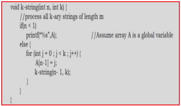
Problem-4 Generate all the strings of length n drawn from 0… k – 1.
Solution: Let us assume we keep the current k-ary string in an array A[0.. n – 1]. Call function kstring(n, k):
Recursion And Back Tracking

Let T(n) be the running time of k – string(n). Then,
Recursion And Back Tracking

Using Subtraction and Conquer Master theorem we get T(n) = O(kn).

Note: For more problems, refer to the String Algorithms chapter.

Problem-5 Finding the length of connected cells of 1s (regions) in a matrix of Os and 1s: Given a matrix, each of which maybe 1 or 0. The filled cells are connected form a region. Two cells are said to be connected if they are adjacent to each other horizontally, vertically, or diagonally. There may be several regions in the matrix. How do you find the largest region (in terms of the number of cells) in the matrix?
Recursion And Back Tracking

Solution: The simplest idea is: for each location traverse in all 8 directions and in each of those directions keep track of maximum region found.
Recursion And Back Tracking


Recursion And Back Tracking


Recursion And Back Tracking


Recursion And Back Tracking

Problem-6 Solve the recurrence T(n) = 2T(n – 1) + 2n.
Solution: At each level of the recurrence tree, the number of problems is double from the previous level, while the amount of work being done in each problem is half from the previous level. Formally, the ith level has 2i problems, each requiring 2n–i work. Thus the ith level requires exactly 2n work. The depth of this tree is n, because at the ith level, the originating call will be T(n – i). Thus the total complexity for T(n) is T(n2n).

Here, in this article, I try to explain Recursion And BackTracking. I hope you enjoy this Recursion And BackTracking article. I would like to have your feedback. Please post your feedback, question, or comments about this article.

Summary:
I hope this post will be helpful to understand the concept of Recursion And Back Tracking
Please share this post with your friends and colleagues.
For any queries please post a comment below.
Happy Coding 😉
Read More
  • Share This:  
  •  Facebook
  •  Twitter
  •  Google+
  •  Stumble
  •  Digg

Master Theorem

 Admin     August 05, 2020     Algorithm, Data Structure     No comments   

In this article, I am going to discuss Master Theorem. Please read our previous article where we discussed Properties of Asymptotic Notations. Here, you will learn what master theorem is and how it is used for solving recurrence relations.

Master Theorem
The master method is a formula for solving recurrence relations of the form:
T(n) = aT(n/b) + f(n),
where,
n = size of input
a = number of subproblems in the recursion
n/b = size of each subproblem. All subproblems are assumed to have the same size. f(n) = cost of the work done outside the recursive call, which includes the cost of dividing the problem and cost of merging the solutions

Here, a ≥ 1 and b > 1 are constants, and f(n) is an asymptotically positive function. An asymptotically positive function means that for a sufficiently large value of n, we have f(n) > 0.

The master theorem is used in calculating the time complexity of recurrence relations (divide and conquer algorithms) in a simple and quick way.

If a ≥ 1 and b > 1 are constants and f(n) is an asymptotically positive function, then the time complexity of a recursive relation is given by

T(n) = aT(n/b) + f(n)
where, T(n) has the following asymptotic bounds:
1. If f(n) = O(nlogb a-ϵ), then T(n) = Θ(nlogb a).
2. If f(n) = Θ(nlogb a), then T(n) = Θ(nlogb a *log n).
3. If f(n) = Ω(nlogb a+ϵ), then T(n) = Θ(f(n)).
ϵ > 0 is a constant.

Each of the above conditions can be interpreted as:
If the cost of solving the sub-problems at each level increases by a certain factor, the value of f(n) will become polynomially smaller than nlogb a. Thus, the time complexity is oppressed by the cost of the last level ie. nlogb a

If the cost of solving the sub-problem at each level is nearly equal, then the value of f(n) will be nlogb a. Thus, the time complexity will be f(n) times the total number of levels ie. nlogb a* log n

If the cost of solving the subproblems at each level decreases by a certain factor, the value of f(n) will become polynomially larger than nlogb a. Thus, the time complexity is oppressed by the cost of f(n).

Solved Example of Master Theorem
T(n) = 3T(n/2) + n2
Here,
a = 3
n/b = n/2
f(n) = n2
logb a = log2 3 ≈ 1.58 < 2
ie. f(n) < nlogb a+ϵ , where, ϵ is a constant.
Case 3 implies here.
Thus, T(n) = f(n) = Θ(n2)

Master Theorem Limitations
The master theorem cannot be used if:
1. T(n) is not monotone. eg. T(n) = sin n
2. f(n) is not a polynomial. eg. f(n) = 2n
3. a is not a constant. eg. a = 2n
4. a < 1

Master Theorem for Divide and Conquer Recurrences
All divide and conquer algorithms (also discussed in detail in the Divide and Conquer chapter) divide the problem into sub-problems, each of which is part of the original problem, and then perform some additional work to compute the final answer. As an example, a merge sort algorithm [for details, refer to Sorting chapter] operates on two sub-problems, each of which is half the size of the original, and then performs O(n) additional work for merging. This gives the running time equation:

T(n) = 2T(n/2) + O(n)

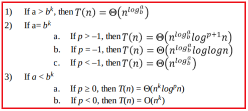
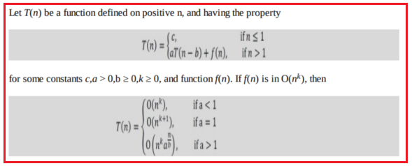
The following theorem can be used to determine the running time of the divide and conquer algorithms. For a given program (algorithm), first, we try to find the recurrence relation for the problem. If the recurrence is of the below form then we can directly give the answer without fully solving it. If the recurrence is of the form ,T(n) = aT (n/b) + Θ(nklogpn) where a ≥ 1,b >1,k ≥ 0 and p is a real number, then:
Master Theorem

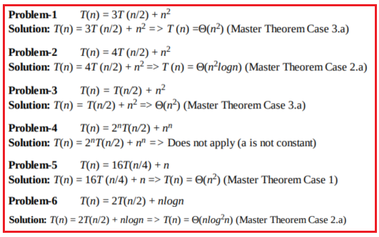
Divide and Conquer Master Theorem: Problems & SolutionsMaster Theorem For each of the following recurrences, give an expression for the runtime T(n) if the recurrence can be solved with the Master Theorem. Otherwise, indicate that the Master Theorem does not apply.
Master Theorem


Master Theorem


Master Theorem

Master Theorem for Subtract and Conquer Recurrences
Master Theorem

A variant of Subtraction and Conquer Master Theorem
The solution to the equation T(n) = T(α n) + T((1 – α)n) + βn, where 0 < α < 1 and β > 0 are constants, is O(nlogn).

Method of Guessing and Confirming
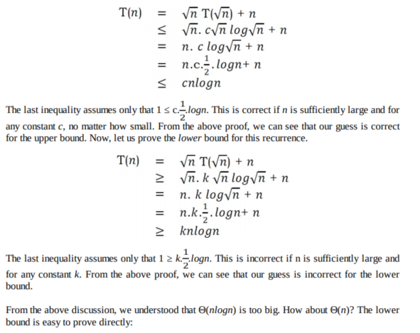
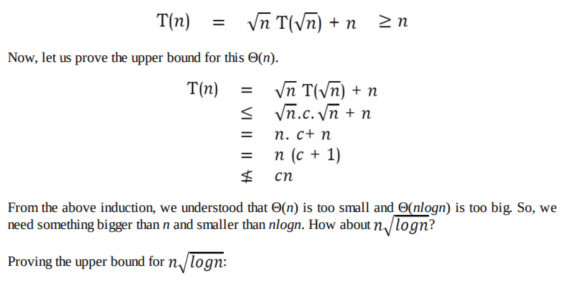
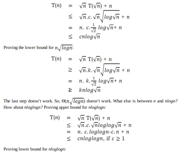
Now, let us discuss a method that can be used to solve any recurrence. The basic idea behind this method is: guess the answer; and then prove it correct by induction.

In other words, it addresses the question: What if the given recurrence doesn’t seem to match with any of these (master theorem) methods? If we guess a solution and then try to verify our guess inductively, usually either the proof will succeed (in which case we are done), or the proof will fail (in which case the failure will help us refine our guess).
Master Theorem
Master Theorem
Master Theorem
Master Theorem
Amortized Analysis
Amortized analysis refers to determining the time-averaged running time for a sequence of operations. It is different from average-case analysis because the amortized analysis does not make any assumption about the distribution of the data values, whereas average case analysis assumes the data are not “bad” (e.g., some sorting algorithms do well on average overall input orderings but very badly on certain input orderings). That is, amortized analysis is a worst-case analysis, but for a sequence of operations rather than for individual operations.

The motivation for amortized analysis is to better understand the running time of certain

techniques, where standard worst-case analysis provides an overly pessimistic bound. Amortized analysis generally applies to a method that consists of a sequence of operations, where the vast majority of the operations are cheap, but some of the operations are expensive. If we can show that the expensive operations are particularly rare we can change them to the cheap operations, and only bound the cheap operations.

The general approach is to assign an artificial cost to each operation in the sequence, such that the total of the artificial costs for the sequence of operations bounds the total of the real costs for the sequence. This artificial cost is called the amortized cost of operation. To analyze the running time, the amortized cost thus is a correct way of understanding the overall running time – but note that particular operations can still take longer so it is not a way of bounding the running time of any individual operation in the sequence.

When one event in a sequence affects the cost of later events:
    One particular task may be expensive. But it may leave data structure in a state that the next few operations become easier.
Example:
Let us consider an array of elements from which we want to find the k the smallest element. We can solve this problem by using sorting. After sorting the given array, we just need to return the kth element from it. The cost of performing the sort (assuming comparison-based sorting algorithm) is O(nlogn). If we perform n such selections then the average cost of each selection is O(nlogn/n) = O(logn). This clearly indicates that sorting once is reducing the complexity of subsequent operations.

In the next article, I am going to discuss Recursion And BackTracking in detail Here, in this article, I try to explain Master Theorem. I hope you enjoy this Master Theorem article. I would like to have your feedback. Please post your feedback, question, or comments about this article.

Summary:
I hope this post will be helpful to understand the concept of Master Theorem
Please share this post with your friends and colleagues.
For any queries please post a comment below.
Happy Coding 😉
Read More
  • Share This:  
  •  Facebook
  •  Twitter
  •  Google+
  •  Stumble
  •  Digg

Properties of Asymptotic Notations

 Admin     August 05, 2020     Algorithm, Data Structure     No comments   

In this article, I am going to discuss Properties of Asymptotic Notations. Please read our previous article where we discussed Asymptotic Notations.

Properties of Asymptotic Notations:
As we have gone through the definition of these three notations let’s now discuss some important properties of those notations.

General Properties :
If f(n) is O(g(n)) then a*f(n) is also O(g(n)) ; where a is a constant.

Example: f(n) = 2n²+5 is O(n²)
then 7*f(n) = 7(2n²+5)
= 14n²+35 is also O(n²)

Similarly, this property satisfies both Θ and Ω notation. We can say
If f(n) is Θ(g(n)) then a*f(n) is also Θ(g(n)); where a is a constant.
If f(n) is Ω (g(n)) then a*f(n) is also Ω (g(n)); where a is a constant.

Reflexive Properties:
If f(n) is given then f(n) is O(f(n)). Example: f(n) = n² ; O(n²) i.e O(f(n))

Similarly, this property satisfies both Θ and Ω notation. We can say
If f(n) is given then f(n) is Θ(f(n)).
If f(n) is given then f(n) is Ω (f(n)).

Transitive Properties :
If f(n) is O(g(n)) and g(n) is O(h(n)) then f(n) = O(h(n)).
Example: if f(n) = n , g(n) = n² and h(n)=n³
n is O(n²) and n² is O(n³) then n is O(n³)

Similarly, this property satisfies both Θ and Ω notation. We can say
If f(n) is Θ(g(n)) and g(n) is Θ(h(n)) then f(n) = Θ(h(n)) .
If f(n) is Ω (g(n)) and g(n) is Ω (h(n)) then f(n) = Ω (h(n))

Symmetric Properties :
If f(n) is Θ(g(n)) then g(n) is Θ(f(n)) .
Example: f(n) = n² and g(n) = n² then f(n) = Θ(n²) and g(n) = Θ(n²)
This property only satisfies for Θ notation.

Transpose Symmetric Properties :
If f(n) is O(g(n)) then g(n) is Ω (f(n)).
Example: f(n) = n , g(n) = n² then n is O(n²) and n² is Ω (n)
This property only satisfies for O and Ω notations.

Some More Properties :
1. If f(n) = O(g(n)) and f(n) = Ω(g(n)) then f(n) = Θ(g(n))
2. If f(n) = O(g(n)) and d(n)=O(e(n))
then f(n) + d(n) = O( max( g(n), e(n) ))

Example: f(n) = n i.e O(n)
d(n) = n² i.e O(n²)
then f(n) + d(n) = n + n² i.e O(n²)

3.If f(n)=O(g(n)) and d(n)=O(e(n))
then f(n) * d(n) = O( g(n) * e(n) )

Example: f(n) = n i.e O(n) d(n) = n² i.e O(n²)
then f(n) * d(n) = n * n² = n³ i.e O(n³)

Commonly used Logarithms and Summations:
Properties of Asymptotic Notations

Commonly used Logarithms and Summations

In the next article, I am going to discuss Master Theorem. Here, in this article, I try to explain the Properties of Asymptotic Notations. I hope you enjoy these Properties of Asymptotic Notations article. I would like to have your feedback. Please post your feedback, question, or comments about this article.

Summary:
I hope this post will be helpful to understand the Properties of Asymptotic Notations
Please share this post with your friends and colleagues.
For any queries please post a comment below.
Happy Coding 😉
Read More
  • Share This:  
  •  Facebook
  •  Twitter
  •  Google+
  •  Stumble
  •  Digg

Asymptotic Notation

 Admin     August 05, 2020     Algorithm, Data Structure     No comments   

In this article, I am going to discuss Asymptotic Notation. Please read our previous article where we discussed the Analysis of Algorithm and why it is important to analyze the algorithm. At the end of this article, you will understand the following pointers in detail with examples.
  1. What are Asymptotic Notations?
  2. Big-O Notation
  3. Omega-Q Notation
  4. Theta-Θ Notation
  5. Why is it called Asymptotic Analysis?
Asymptotic Notation
Having the expressions for the best, average, and worst cases, for all three cases we need to identify the upper and lower bounds. To represent these upper and lower bounds, we need some kind of syntax, and that is the subject of the following discussion. Let us assume that the given algorithm is represented in the form of function f(n).

The following 3 asymptotic notations are mostly used to represent the time complexity of algorithms.

Big-O Notation [Upper Bounding Function]
This notation gives the tight upper bound of the given function. Generally, it is represented as f(n)= O(g(n)). That means, at larger values of n, the upper bound of f(n) is g(n). For example, if f(n)= n4 + 100n2 + 10n + 50 is the given algorithm, then n4 is g(n). That means g(n) gives the maximum rate of growth for f(n) at larger values of n.
Big-O Notation [Upper Bounding Function]

O(g(n)) = { f(n): there exist positive constants c and n0 such that 0 <= f(n) <= c*g(n) for all n >= n0 }.
The statement f(n) = O(g(n)) states only that g(n) is an upper bound f(n) for all n , n >= n0 .
Note: In below Big- 0 Examples n0 denoted by n0.

Big-O Examples

Example-1 Find upper bound for f(n) = 3n + 8
Solution: 3n + 8 ≤ 4n, for all n ≥ 8
3n + 8 = O(n) with c = 4 and n0 = 8

Example-2 Find upper bound for f(n) = n2 + 1
Solution: n2 + 1 ≤ 2n2 , for all n ≥ 1
n2 + 1 = O(n2) with c = 2 and n0 = 1

Example-3 Find upper bound for f(n) = n4 + 100n2 + 50 Solution: n4 + 100n2 + 50 ≤ 2n4, for all n ≥ 11
n4 + 100n2 + 50 = O(n4) with c = 2 and n0 = 11

Example-4 Find upper bound for f(n) = 2n3 – 2n2
Solution: 2n3 – 2n2 ≤ 2n3, for all n > 1
2n3 – 2n2 = O(n3) with c = 2 and n0 = 1

Example-5 Find upper bound for f(n) = n
Solution: n ≤ n, for all n ≥ 1
n = O(n) with c = 1 and n0 = 1

Example-6 Find upper bound for f(n) = 410 Solution: 410 ≤ 410, for all n > 1
410 = O(1) with c = 1 and n0 = 1

No Uniqueness?
There is no unique set of values for n0 and c in proving the asymptotic bounds. Let us consider, 100n + 5 = O(n). For this function, there are multiple n0 and c values possible.

Solution1: 100n + 5 ≤ 100n + n = 101n ≤ 101n, for all n ≥ 5, n0 = 5 and c = 101 is a solution. Solution2: 100n + 5 ≤ 100n + 5n = 105n ≤ 105n, for all n > 1, n0 = 1 and c = 105 is also a solution.

Omega-Q Notation [Lower Bounding Function]
Similar to the O discussion, this notation gives the tighter lower bound of the given algorithm and we represent it as f(n) = Ω(g(n)). That means, at larger values of n, the tighter lower bound of f(n) is g(n). For example, if f(n) = 100n2 + 10n + 50, g(n) is Ω(n2).
Omega-Q Notation [Lower Bounding Function]

For a given function g(n), we denote by Ω(g(n)) the set of functions. Ω (g(n)) = {f(n): there exist positive constants c and n0 such that 0 <= c*g(n) <= f(n) for all n >= n0}.

Omega (Ω) Examples
Example-1 Find lower bound for f(n) = 5n2.
Solution: ∃ c, n0 Such that: 0 ≤ cn2≤ 5n2 ⇒ cn2 ≤ 5n2 ⇒ c = 5 and n0 = 1 5n2 = Ω(n2) with c = 5 and n0 = 1

Example-2 Prove f(n) = 100n + 5 ≠ Ω(n2).
Solution: ∃ c, n0 Such that: 0 ≤ cn2 ≤ 100n + 5 => 100n + 5 ≤ 100n + 5n(∀n ≥ 1) = 105n => cn2 ≤ 105n ⇒ n(cn – 105) ≤ 0 Since n is positive ⇒cn – 105 ≤0 ⇒ n ≤105/c ⇒ Contradiction: n cannot be smaller than a constant

Theta-Θ Notation [Order Function]
The theta notation bound functions from above and below, so it defines exact asymptotic behavior. A simple way to get Theta notation of an expression is to drop low order terms and ignore leading constants. For example, consider the following expression.

3n3 + 6n2 + 6000 = Θ(n3)

Dropping lower order terms is always fine because there will always be a n0 after which Θ(n3) has higher values than Θn2) irrespective of the constants involved.
Theta-Θ Notation [Order Function]

For a given function g(n), we denote Θ(g(n)) is following set of functions.

Θ(g(n)) = {f(n): there exist positive constants c1, c2 and n0 such that 0 <= c1*g(n) <= f(n) <= c2*g(n) for all n >= n0}

The above definition means, if f(n) is theta of g(n), then the value f(n) is always between c1*g(n) and c2*g(n) for large values of n (n >= n0). The definition of theta also requires that f(n) must be non-negative for values of n greater than n0.

Theta (Θ) Examples

Example 1 Prove n ≠ Θ(n2)
Solution: c1n2 ≤ n ≤ c2n2 ⇒ only holds for: n ≤ 1/c1
n ≠ Θ(n2)

Example 2 Prove 6n3 ≠ Θ(n2)
Solution: c1n2≤ 6n3 ≤ c2n2 ⇒ only holds for n ≤ c2/6
6n3 ≠ Θ(n2)

Example 3 Prove n ≠ Θ(logn)
Solution: c1logn ≤ n ≤ c2logn ⇒ c2 ≥ n/log n, ∀ n ≥ n0 – Impossible

Important Notes
For analysis (best case, worst case, and average), we try to give the upper bound (O) and lower bound (Ω) and average running time (Θ). From the above examples, it should also be clear that, for a given function (algorithm), getting the upper bound (O) and lower bound (Ω) and average running time (Θ) may not always be possible. For example, if we are discussing the best case of an algorithm, we try to give the upper bound (O) and lower bound (Ω) and average running time(Θ).

In the remaining chapters, we generally focus on the upper bound (O) because knowing the lower-bound (Ω) of an algorithm is of no practical importance, and we use the Θ notation if the upper bound (O) and lower bound (Ω) are the same.

Why is it called Asymptotic Analysis?
From the discussion above (for all three notations: worst case, best case, and average case), we can easily understand that in every case for a given function f(n) we are trying to find another function g(n) which approximates f(n) at higher values of n. That means g(n) is also a curve which approximates f(n) at higher values of n.

In mathematics, we call such a curve an asymptotic curve. In other terms, g(n) is the asymptotic curve for f(n). For this reason, we call algorithm analysis asymptotic analysis.

In the next article, I am going to discuss Properties of Asymptotic Notations. Here, in this article, I try to explain Asymptotic Notation. I hope you enjoy this Asymptotic Notation article. I would like to have your feedback. Please post your feedback, question, or comments about this article.

Summary:
I hope this post will be helpful to understand the concept of Asymptotic Notation
Please share this post with your friends and colleagues.
For any queries please post a comment below.
Happy Coding 😉
Read More
  • Share This:  
  •  Facebook
  •  Twitter
  •  Google+
  •  Stumble
  •  Digg

Analysis of Algorithm

 Admin     August 05, 2020     Algorithm, Data Structure     No comments   

In this article, I am going to discuss the Analysis of Algorithm as well as why it is important to Analysis the Algorithm. Please read our previous article where we gave a brief introduction to Data Structure and Algorithm. At the end of this article, you will understand the following pointers in detail.
  1. Why Analysis of Algorithm?
  2. The goal of Analysis of Algorithms.
  3. What is Running Time Analysis?
  4. How to compare Algorithms?
  5. Does Asymptotic Analysis always work?
  6. What is the Rate of Growth?
  7. Types of Analysis
Why Analysis of Algorithm?
Algorithm analysis helps to determine the best among others in terms of time and space consumed. For example:- Going from one place to another, there are various ways to travel. Like Bus, Train, Flight, Car, etc.

But we will select the best mode which is cost-efficient and time-consuming, depends on the situation. Similarly, In computer science to sort an array there are various ways or algorithms like insertion sort, selection sort, quick sort, merge sort, etc.

The goal of Analysis of Algorithms
the Goal of analysis of algorithms is to compare algorithms (for solutions) mainly in terms of running time but also in terms of other factors (e.g. memory, developers effect, etc.)

What is Running Time Analysis?
It is the processing time vs size of the input. The input may be of different types based on problems. Commons inputs are
  1. Size of array
  2. Number of elements in a matrix
  3. Polynomial degree
  4. Numbers of bits in binary representation
  5. Edges and Vertices in a graph
How to compare Algorithms?
One native way of doing this is – implement both the algorithms and run the two programs on your computer for different inputs and see which one takes less time. There are many problems with this approach to the analysis of algorithms.
  1. It might be possible that for some inputs, the first algorithm performs better than the second. And for some inputs, second performs better.
  2. It might also be possible that for some inputs, first algorithm perform better on one machine and the second works better on other machines for some other inputs.
Asymptotic Analysis is a big idea that handles the above issues in analyzing algorithms. In Asymptotic Analysis, we evaluate the performance of an algorithm in terms of input size (we don’t measure the actual running time). We calculate, how the time (or space) taken by an algorithm increases with the input size.

This kind of comparison is independent of machine time, programming type, etc.

Example to understand this concept:
For example, let us consider the search problem (searching a given item) in a sorted array. One way to search is Linear Search (order of growth is linear) and the other way is Binary Search (order of growth is logarithmic).

To understand how Asymptotic Analysis solves the above-mentioned problems in analyzing algorithms, let us say we run the Linear Search on a fast computer A and Binary Search on a slow computer B and we pick the constant values for the two computers so that it tells us exactly how long it takes for the given machine to perform the search in seconds.

Let’s say the constant for A is 0.2 and the constant for B is 1000 which means that A is 5000 times more powerful than B. For small values of input array size n, the fast computer may take less time. But, after a certain value of input array size, the Binary Search will definitely start taking less time compared to the Linear Search even though the Binary Search is being run on a slow machine.

The reason is the order of growth of Binary Search with respect to input size is logarithmic while the order of growth of Linear Search is linear. So the machine-dependent constants can always be ignored after a certain value of input size.

Here are some running times for this example:
Linear Search running time in seconds on A: 0.2 * n
Binary Search running time in seconds on B: 1000*log(n)

Analysis of Algorithm

Does Asymptotic Analysis always work?
Asymptotic Analysis is not perfect, but that’s the best way available for analyzing algorithms. For example, say there are two sorting algorithms that take 1000nLogn and 2nLogn time respectively on a machine. Both of these algorithms are asymptotically the same (order of growth is nLogn). So, With Asymptotic Analysis, we can’t judge which one is better as we ignore constants in Asymptotic Analysis.

Also, in Asymptotic analysis, we always talk about input sizes larger than a constant value. It might be possible that those large inputs are never given to your software and an algorithm that is asymptotically slower, always performs better for your particular situation. So, you may end up choosing an algorithm that is Asymptotically slower but faster for your software.

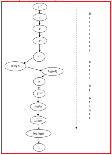
What is the Rate of Growth? The rate at which running time increases as a function of input is called the rate of growth.

We know that for the growth of a function, the highest order term matters the most e.g., the term c1n2 in the function c1n2+c2n+c3 and thus we can neglect the other terms and even the coefficient of the highest order term i.e., c1 (assuming coefficients are neither too large nor too small).

Even with these approximations, we will be able to know about the rate of the growth of our function and this is enough information to keep in our mind while developing an algorithm.

Commonly used rate of Growths in decreasing order
What is the Rate of Growth?

Commonly used rate of Growths in decreasing order

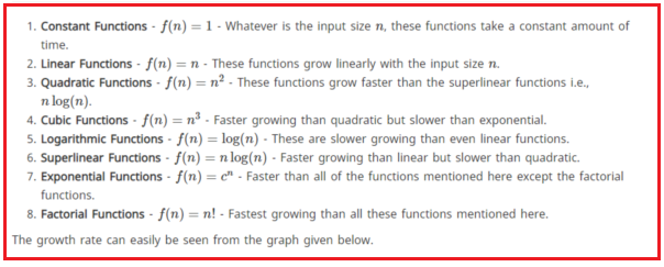
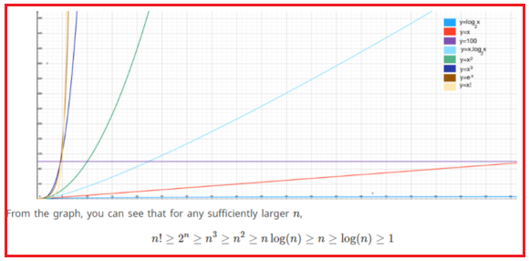
Commonly used functions and Their comparison:
Commonly used functions and Their comparison

and the problem
Types of Analysis

Types of Analysis
To analyze the given algorithm we need to know on what inputs the algorithm is taking less time (performing well) and on what inputs the algorithm is taking a huge time. We know that an algorithm can be represented in the form of expression. That means we represent the algorithm with multiple expressions: one for the case where it is taking less time and others for the case where it is taking more time. In general-

Worst Case:- Defines the input for which the algorithm takes a huge time. Input is the one for which the algorithm runs slower.

Best Case:- Defines the input for which algorithm takes the lowest time. Input is the one for which algorithm works fastest.

Average Case:- Provides a prediction about the running time of the algorithm. Assumes that the input is random.

Lower Bound <= Average Time <= Upper Bound
For a given algorithm, we can represent best, worst, and average cases in the form of expression.

Example:- f(n) = n2 + 500, for worst-case
f(n) = n + 100n + 500, for best case

Similarly, we can define the average case too.

In the next article, I am going to discuss Asymptotic Notation. Here, in this article, I try to explain the Analysis of Algorithm. I hope you enjoy this Introduction Analysis of Algorithm article. I would like to have your feedback. Please post your feedback, question, or comments about this article.

Summary:
I hope this post will be helpful to understand the Analysis of Algorithm
Please share this post with your friends and colleagues.
For any queries please post a comment below.
Happy Coding 😉
Read More
  • Share This:  
  •  Facebook
  •  Twitter
  •  Google+
  •  Stumble
  •  Digg

Sunday, August 2, 2020

Introduction to Data Structure and Algorithm

 Admin     August 02, 2020     Algorithm, Data Structure     No comments   

In this article, I am going to give you a brief introduction to Data Structure and Algorithm. At the end of this article, you will understand what is Data Structure and Algorithm, its type, and why we need data structure and algorithm as well as Variables and Data Types.

Variables:
let's take an simple mathematical equation.
x + y – 10 = 20 eq1.1
For now, we don’t need to worry about the equation. As we all can observe, the eq1.1 has some names which hold values(data). Similarly, in programming something required to hold data, and we called them variables. In eq1.1, x & y are variables which holds some data.

Data Types:
In eq1.1, x & y holds some data and the data may be integers or floats like 0,1, 0.5, -6.4 , -2 etc. A data type is a set of some predefined values like Integers, Floating points, character, strings etc. There are two types of data types.
  1. System – defined Data types (also called as Primitive data types)
  2. User – defined Data types
System Defined Data Types
Primitive data type defined by the system .It is provided by programming language. Example – int, float, char, bool, etc.

Allocation of bits for each primitive data type depends on programming language, operating system, and compiler. Different programming language may allocate different size for the same primitive data type.

User-Defined Data Types
In many cases to solve a problem, system-defined data types are not enough. To overcome this situation many programming languages allow the users to define their own data type called user define data types.

Data Structures in C/C++ and classes in java are good examples. Generally, user-defined data type is a combination of much primitive data type.
struct usrdef {
     int sysdef1;
    float sysdef2;
    bool sysdef3;
};
Data Structure
In computer science, a data structure is a data organization, management, and storage format that enables efficient access and modification. More precisely, a data structure is a collection of data values, the relationships among them, and the functions or operations that can be applied to the data.

In simple words, a data structure is a way of storing and organizing data so that it can be used efficiently.

Types of Data Structure:
Data Structure classified mainly into two types.
Linear Data Structure:- A Linear data structure have data elements arranged in a sequential manner and each member element is connected to its previous and next element.
Example:- LinkedList, stacks, queue, trees, graphs, etc.

Non-Linear Data Structures:- A non-linear data structure has no set sequence of connecting all its elements and each element can have multiple paths to connect to other elements.
Example:- Trees, Graphs.

For a better understanding of the classification of data structure please have a look at the following diagram.
Types of Data Structure

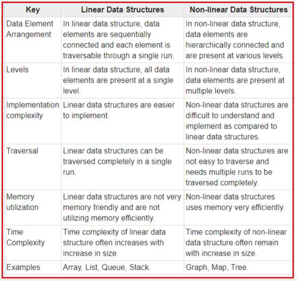
Key Differences between Linear and Non-Linear Data Structure
Differences between Linear and Non - Linear Data Structure

Advantages of Data Structures or why we need Data Structure?
We need data structures, few of them are as follows:
  1. They are essential ingredients in creating a fast and powerful algorithm.
  2. They help to manage and organize data.
  3. They make code cleaner and easier to understand.
Abstract Data Types
Basic operation like addition, multiplication, division, subtraction supported by primitive data type but for the user-defined data type, we need to define operations. such operations can be defined at the time of implementation.

In general, user-defined data types are defined along with their operations. The combination of data structures along with their operations is called Abstract Data Types (ADTs). It mainly consists of two parts.
  1. Declaration of data
  2. Declaration of operations
What is an Algorithm?
An algorithm is a set of one – by – one instruction to solve a particular problem.

Example:- Adding two numbers given by the users
Step 1: Start
Step 2: Declare variables no1, no2, and summation.
Step 3: Read values no1 and no2 that is provided by the user.
Step 4: Add no1 and no2 and assign the result to summation.
             summation ← num1 + num2
Step 5: Display summation
Step 6: Stop
Properties of a good algorithm
  1. Input and output should be clearly defined.
  2. Each step in the algorithm should be clear and unambiguous.
  3. Algorithms should be most effective among many different ways to solve a problem.
The algorithm should be written in such a way that it can be used in different programming languages. No coding is allowed.

In the next article, I am going to discuss the Analysis of Algorithm in detail. Here, in this article, I try to give a brief introduction to Data Structure and Algorithm and I hope you enjoy this article. I hope you enjoy this Introduction to Data Structure and Algorithm article. I would like to have your feedback. Please post your feedback, question, or comments about this article.

Summary:
I hope this post will be helpful to understand the Introduction to Data Structure and Algorithm
Please share this post with your friends and colleagues.
For any queries please post a comment below.
Happy Coding 😉
Read More
  • Share This:  
  •  Facebook
  •  Twitter
  •  Google+
  •  Stumble
  •  Digg
Older Posts

Join us on Telegram

Loved Our Blog Posts? Subscribe To Get Updates Directly To Your Inbox

Like us on Facebook

Popular Posts

  • What is Dependency Injection(DI)
    Hi friends! Today we are going to learn about Dependency Injection and in our last session we have come across Static classes and where it s...
  • C# Programming Examples on Sorting
    Today i am going to tell you some of the Sorting programming questions in C#. Q1- Write a C# program to perform Selection sort. Ans:  Sel...
  • Calling Web API Service in a Cross-Domain Using jQuery AJAX
    In this article, I am going to discuss Calling Web API Service in a Cross-Domain Using jQuery AJAX . Please read our previous article befor...
  • ViewBag in ASP.NET Core MVC
    In this article, I am going to discuss the use of ViewBag in ASP.NET Core MVC application with examples. Please read our previous article ...
  • Recursion And Back Tracking
    In this article, I am going to discuss Recursion And BackTracking in detail. Please read our previous article where we discussed Master Th...
  • What is Abstract Class and When we should use Abstract Class
    Hi friends! In our previous sessions we have seen  Difference Between Class and Struct . And in our last session  we learnt Usability of Sec...
  • Binary to Decimal Conversion in C# with Examples
    In this article, I am going to discuss the Binary to Decimal Conversion in C# with some examples. Please read our previous article where w...

Blog Archive

Contact Form

Name

Email *

Message *

Tags

.Net .Net Core .Net Core MVC Algorithm Angular Anonymous Types Asp.Net Asp.Net MVC Blazor C# Data Structure Database Design Patterns Entity Framework Entity Framework Core Filters Interview Question Management Studio Programming Programs SQL Server SSMS Web API

Copyright © C# Techtics | All Right Reserved.

Protected by Copyscape